

 Sviatlana Staleuskaya
How machine learning can improve trading bots profitability on Crypto markets.


Machine learning methods are widely adopted for algorithmic trading and are becoming a staple product in the modern financial market. The purpose of this research is to evaluate a filtration method to improve a trading strategy performance by eliminating unnecessary trade signals. The implementation is inspired by Marcos Lopez de Prado's ideas outlined in his book “Advances in Financial Machine Learning”. Thorough back-testing experiments carried out in QuantOffice Cloud have revealed that this approach can reduce the number of unprofitable trades sent by a strategy significantly, thereby mitigating losses in the form of exchanges’ commissions.
This research paper has been created by Aliaksandr Yuretski, Sviatlana Staleuskaya, and Isaac Gorelik - members of the QuantOffice Cloud team.
Introduction
The primary purpose of this experiment is to determine whether the machine learning techniques can improve the performance of a momentum-based trading strategy. In our experiments, we use a trading strategy adapted from Dissecting Investment Strategies in the Cross-Section and Time Series, by Baz et. al (2015). Our primary goal is to improve the performance of this strategy by training an algorithm to filter out the detrimental or unnecessary trades which do not generate returns.
The secondary goal is to explore the QuantOffice Cloud capabilities as Jupyter Lab-based strategy development and testing studio especially in conjunction with machine learning technologies.
Baseline Trading Strategy
The strategy generates trading signals, ranging (-1, 1), by taking three values’ average derived from differences of EMAs with various time periods. We have simplified it for this experiment by using a uniform bet size and discrete signals: the signal acquires a value of ±1 if its magnitude exceeds a certain threshold; otherwise, the signal is set to 0. Our baseline trading strategy consists of six strategy instances running concurrently, each tuned to maximize performance. The strategy details are not covered in this research. We have developed the strategy in Python programming language and backtested it on the QuantOffice Cloud platform which offers a powerful set of APIs and the development environment allowing to focus on core activities such as design and prototyping. Backtested strategy can be easily run live on real or paper accounts. Trading logic is straightforward and placed in a single method:
self.avrgS.add(current_price)
self.avrgL.add(current_price)
self.avrgC2.add(current_price * current_price)
self.avrgC.add(current_price)

if self.avrgS.stable() and self.avrgL.stable() and \
       self.avrgC.stable() and self.avrgC2.stable():
   Z = (self.avrgS.value() - self.avrgL.value()) / math.sqrt(
       self.avrgC2.value() - self.avrgC.value() * self.avrgC.value())
   self.avrgZ.add(Z)
   self.avrgZ2.add(Z * Z)
   if self.avrgZ.stable() and self.avrgZ2.stable():
       z_score = (Z - self.avrgZ.value()) / math.sqrt(
           self.avrgZ2.value() - self.avrgZ.value() * self.avrgZ.value())
       fctr = (z_score * math.exp(-0.25 * z_score * z_score) /
               (math.sqrt(2.0) * math.exp(-0.5)))

       signal = 1 if fctr > self.threshold \
else (-1 if fctr < -self.threshold else 0)

       update_last_signal(instr, signal)
       if instr.portfolio_executor.draw_indicators:
           self.line_fctr.draw(current_time, fctr)

       if not instr.is_warmup_mode():
           if signal == 1 and \
                   abs(position_size(instr, portfolio = self.portfolio)) <  instr.min_order_size:
               on_buy_signal(instr, "Open Long position", portfolio = self.portfolio)
               self.hold_periods = 0
           elif signal == -1 and \
                   abs(position_size(instr, portfolio = self.portfolio)) < instr.min_order_size:
               on_sell_signal(instr, "Open Short position", portfolio = self.portfolio)
               self.hold_periods = 0
We have backtested the strategy in JupyterHub so all the parameters are managed in Jupyter Notebook files:
symbols = 'BTCUSD LTCUSD ETHUSD'
price_stream = 'KRAKEN_BARS'
bar_size=BarSize(BarUOM.Minute, 1)
start_time = "2019-03-01T00:00:00"
end_time = "2021-10-19T00:00:00"

input_parameters.initial_cap = 18000
# bet size is 1000$
input_parameters.bet_size = 1000
input_parameters.generate_reports = True
input_parameters.holding_period = 60*24 # bars
PortfolioExecutor.instances = [StrategyInstance(4*60, 24*60, 0.99961, "p1"),
                              StrategyInstance(60, 24*60, 0.99845, "p2"),
                              StrategyInstance(24*60, 5*24*60, 0.99999, "p3"),
                              StrategyInstance(5, 5*24*60, 0.99967, "p4"),
                              StrategyInstance(60, 5*24*60, 0.99994, "p5"),
                              StrategyInstance(15, 5*24*60, 0.99999, "p6"),
For this experiment, we use Ethereum, Litecoin, and Bitcoin price data from Kraken exchange, which is available for QuantOffice Cloud users out of the box as well as a back-testing strategy for a two-year period. Back-testing results are presented in Figure 1 and Table 1.
Figure 1.: Strategy’s realized PnL backtested on BTCUSD, LTCUSD, ETHUSD from Mar 2019 to Oct 2021.
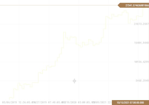
Table 1.: Strategy’s performance.
| Parameters | All Trades | Long Trades | Short Trades |
|---|---|---|---|
| Net Profit/Loss | 27323.56 | 27757.08 | -433.522 |
| Total Profit | 125140.8 | 67898.73 | 57242.03 |
| Total Loss | -97817.2 | -40141.6 | -57675.6 |
| Max Drawdown | -5617.29 | -3651.31 | -9881.1 |
| Return/Drawdown Ratio | 4.8642 | 7.602 | -0.0439 |
| Max Drawdown Duration | 271 day(s) | 139 day(s) | 584 day(s) |
| Information Ratio | 1.2509 | 1.8731 | -0.0184 |
| All Trades # | 6414 | 3169 | 3245 |
| Profitable Trades Ratio | 0.5123 | 0.5589 | 0.4669 |
| Winning Trades # | 3286 | 1771 | 1515 |
| Losing Trades # | 3128 | 1398 | 1730 |
| Average Trade | 4.26 | 8.7589 | -0.1336 |
| Avg Profit Per Trade (bps) | 42.5064 | 87.2088 | -1.3359 |
| Average Winning Trade | 38.083 | 38.3392 | 37.7835 |
| Average Losing Trade | -31.2715 | -28.7136 | -33.3385 |
| Avg. Win/Avg. Loss Ratio | 1.2178 | 1.3352 | 1.1333 |
| Max Conseq. Winners | 38 | 29 | 34 |
| Max Conseq. Losers | 49 | 38 | 39 |
Machine Learning Application
The experiment’s goal is to train the classifier to filter out the detrimental trading signals provided by the strategy. We use QuantOffice’s library, which gives access to the classifier in conjunction with the existing strategy, and train this model as we gather enough data to generate the necessary factors (figure 2).
Figure 2.: Applying machine learning methods to filtering trading strategy signals.

We start by labeling the training set using a modification of the Marcos Lopez de Prado three-barrier method with a 24-hour horizon and some threshold. Strategy’s open position points are considered as learning objects. The signal gets a label of ±1 (depending on the sign of the return) if the returned absolute value is greater than the threshold; otherwise, the label is 0.
Features module of the library handles the extraction of factors, their normalization, and dimension reduction. Factors include the data derived from the price of each instrument (considering price deviations over various time intervals). We use momentum-type series, logarithmical returns, and volatility calculated with different lags as additional factors. Autoencoder and principal component analysis are used as algorithms to reduce the dimensionality of the factor space.
Estimators module contains a set of built-in classifiers such as
- Random Forest (RF)
- XGBoost
- Multilayer Perceptron (MLP)
- Support Vector Machine (SVM)
- K-Nearest Neighbors (kNN)
Classifiers can be added from the standard Python library (for example, scikit-learn: machine learning in Python — scikit-learn 1.0 documentation) or created by the user. During our experiments, we have discovered that optimal factors can be extracted based on the price data aggregated over the course of minimum 30 consecutive days. Meaning that the model can be trained having received the above-mentioned dataset. Having met these conditions, we use the model for 24 hours to predict which signals to keep and which to reject. After 24 hours, the model is retrained using the most recent 30 days of price data (and any indicators of interest) to rebuild the factors and make a prediction for another 24 hours. This cycle continues until the back-testing ends. For example, let’s consider a back-testing period starting from the 1st of January until the 28th of February.
- On the 31st of January, the model is trained on the price data for 30 days (1st - 30th of January). This model is then used to make a prediction for the 31st of January.
- On the 1st of February, the model is trained using factors from the 2nd – 31st of January and so on.
Data is randomly separated into training and test sets during the training. We use 5 folds cross-validation to find the parameters which minimize the total validation set error. The prediction is made only when the model provides a nonzero signal to buy or sell (since the role of the classifier is to filter the detrimental trading signals).
Results
The results of the tested classifiers are presented in Table 2 and Figure 3. Support vector machine and multilayer perceptron classifiers showed better performance. All classifiers that we used in our experiments are specified in backtesting.ipynb.
Figure 3.: PnL of the strategy with SVM-filtered signals from Mar 2019 to Oct 2021.

| Parameters | Base | kNN | MPL | RF | SVM | XGBoost |
|---|---|---|---|---|---|---|
| Net Profit/Loss | 27323.56 | 24443.6 | 24967.18 | 23492.63 | 27598.96 | 22324.94 |
| Total Profit | 125140.8 | 92431.48 | 72167.95 | 91177.17 | 70799.8 | 104864 |
| Total Loss | -97817.2 | -67987.9 | -47200.8 | -67684.5 | -43200.8 | -82539 |
| Max Drawdown | -5617.29 | -3653.57 | -2847.7 | -4092.29 | -2211.13 | -5295.64 |
| Return/Drawdown Ratio | 4.8642 | 6.6903 | 8.7675 | 5.7407 | 12.4819 | 4.2157 |
| Max Drawdown Duration | 271 day(s) | 165 day(s) | 190 day(s) | 128 day(s) | 189 day(s) | 237 day(s) |
| Information Ratio | 1.2509 | 1.4392 | 1.6941 | 1.4249 | 1.8807 | 1.1933 |
| All Trades # | 6414 | 4739 | 3415 | 4669 | 3273 | 5484 |
| Profitable Trades Ratio | 0.5123 | 0.5151 | 0.5388 | 0.5108 | 0.5448 | 0.5055 |
| Winning Trades # | 3286 | 2441 | 1840 | 2385 | 1783 | 2772 |
| Losing Trades # | 3128 | 2298 | 1575 | 2284 | 1490 | 2712 |
| Average Trade | 4.26 | 5.158 | 7.311 | 5.0316 | 8.4323 | 4.0709 |
| Avg Profit Per Trade (bps) | 42.5064 | 51.4458 | 72.8522 | 50.157 | 84.0269 | 40.6192 |
| Average Winning Trade | 38.083 | 37.8662 | 39.2217 | 38.2294 | 39.7082 | 37.8297 |
| Average Losing Trade | -31.2715 | -29.5857 | -29.9687 | -29.6342 | -28.9939 | -30.4347 |
| Avg. Win/Avg. Loss Ratio | 1.2178 | 1.2799 | 1.3088 | 1.29 | 1.3695 | 1.243 |
| Max Conseq. Winners | 38 | 32 | 29 | 29 | 29 | 35 |
| Max Conseq. Losers | 49 | 31 | 26 | 29 | 25 | 35 |
The results show the spread in PnL among the filtered strategies (22-27k as opposed to 27k). This is caused by the fact that the signal filtration decreases the total number of signals while keeping the average profit in bps and information ratio higher. As a result of our back-testing experiments, we have provided supportive evidence to the hypothesis that machine learning techniques can improve trading strategy performance.
Conclusion
In this research, we have studied how a simplified trading strategy implemented on the QuantOffice Cloud platform can be optimized using machine learning algorithms such as random forest, XGBoost, multilayer perceptron, support vector machine, k-nearest neighbors. We have demonstrated the possibility of using these methods to improve the sample trading strategy performance by adding new factors and filtering signals.
References
- Baz, J., Granger, N., Harvey, C. R., Le Roux, N., Rattray, S. (December 4, 2015). Dissecting Investment Strategies in the Cross Section and Time Series Available at SSRN: https://ssrn.com/abstract=2695101, or https://www.cmegroup.com/education/files/dissecting-investment-strategies-in-the-cross-section-and-time-series.pdf
- Dixon, M.F., Klabjan, D., & Bang, J.H. (2015). Implementing deep neural networks for financial market prediction on the Intel Xeon Phi. Proceedings of the 8th Workshop on High-Performance Computational Finance.
- Lopez de Prado, M. (2018). Advances in financial machine learning. John Wiley & Sons.
- QuantOffice Cloud. Available at QuantOffice Cloud.
Sviatlana Staleuskaya